Exploratory Spatial Data Analysis: STATA Application (1)

In spatial econometrics, before we run the model, we need to compute descriptive statistics, as in the non-spatial econometrics approach. In spatial econometrics, there is an extension beyond describing data (mean, maximum, minimum, and standard deviation). It is called Exploratory Spatial Data Analysis (ESDA) and uses map visualisation to identify patterns. Also, we need to assess spatial autocorrelation using Global Moran’s I and the presence of local clusters. The formula for Moran’s I is :

I = \frac{n}{\sum_{i}^{n} \sum_{j}^{n} w_{ij}} . \frac{\sum_{i}^{n}\sum_{j}^{n} w_{ij}(x_i – \bar{x})(x_j – \bar{x})} {\sum_{i}^{n} (x_i – \bar{x})^2}

where :

$n$ = The total number of spatial units (e.g., villages, districts, or regions)
$x_i$ = The value of the variable of interest in spatial unit $i$
$x_j$ =The value of the variable of interest in spatial unit $j$
$\bar{x}$ = The mean of the variable across all spatial units.
$w_{ij}$ = The spatial weight between units i and j, indicating whether (and how strongly) the two units are spatially connected. Standard definitions include contiguity-based (shared borders) or distance-based weights
$\sum_{i}^{n} \sum_{j}^{n} w_{ij}$ = The sum of all spatial weights
Numerator: The spatial covariance, measuring the co-movement of values across neighbouring locations.
Denominator: The overall variance of the variable.

Why use Moran I ?

The Global Moran’s I is used as a metric for global spatial autocorrelation, and it is mostly used for aerial data, along with ratio or interval data (Grekousis, 2020). As inferential statistics, Global Moran’s I is interpreted based on the expected value from the above equation under the hypothesis :

$H_0 =$ No spatial autocorrelation (spatial randomness)

The evaluation of this hypothesis is using $p$ -value and a $z$ -score. The expected value for a random pattern is :

E({I}) = -1 / n-1

where n denotes the number of spatial units.

Interpret Moran’s I value

Moran’s I ranges from −1 to +1. A value close to +1 indicates strong positive spatial autocorrelation; a value close to −1 indicates strong negative spatial autocorrelation.
$I > 0$ = positive spatial autocorrelation, neighbouring units tend to have similar values (high–high or low–low), so the pattern is clustered.
<math data-latex="I I<0I < 0 = negative spatial autocorrelation, neighbouring units tend to have dissimilar values (high near low), so the pattern is dispersed or checkerboard – like.
$I \approx 0$ (or close to the expected value $-1/(n-1)$ , no clear spatial pattern, approximately random.

Role of Expected I, z-score and p-value

Expected I is the value of Moran’s I under the null hypothesis of complete spatial randomness; for many cases, it equals $-1/(n-1)$
The z-score is $z = \frac{I - E [I]}{\sqrt{V a r (I)}}$ and tells how many standard deviations the observed I is away from what is expected under randomness.
The p-value indicates the probability of obtaining an I at least as extreme as the observed one under the null hypothesis that the pattern is random; a small p-value (e.g., < 0.05) indicates the spatial pattern is statistically significant.

Suppose the result of Moran’s I :

Moran’s I = 0.35
Expected I = −0.01
z-score = 4.2
p-value = 0.00003

Then

The p-value < 0.05, we reject the null hypothesis of spatial randomness, indicating significant spatial autocorrelation.
The value of I is positive (0.35) and clearly larger than the expected value (-0.01). This indicates that the pattern is clustered: neighbouring areas tend to have similar values (e.g., groups of high-poverty districts close to each other and groups of low-poverty districts close to each other.

The STATA Code for Moran’s I.

I use command “genmsp” from from Maurizio Pisati .I replicated it for poverty data in Java Island, Indonesia at the ADM2 level in 2024. In practical terms, for a variable $Y$ , genmsp will typically:

Standardize $Y$ to create a z‑score (e.g. std_Y).
Compute the spatial lag of the standardized variable using the specified spatial weights matrix (e.g. Wstd_Y).
Run local Moran’s I for each observation and save the local I, z‑score, and p‑value (e.g. Ii_Y, z_Y, pval_Y).
Generate a categorical variable (often called something like msp_Y) that classifies each observation into Moran scatterplot quadrants and LISA cluster types: High–High, Low–Low, High–Low, Low–High, or not significant, based on a chosen p‑value threshold (e.g. 0.05)

References

Stata Forum
Pisati, 2012. Exploratory spatial data analysis using Stata
Grekousis, 2020. Spatial Analysis Methods and Practice Describe – Explore – Explain through GIS.

The Practice : STATA Application.

In the application, you just replace the directory path with your directory. All data is available in my Github, so the do file will automatically execute it direclty. Just run it.


clear 
set more off
capture close log

cd "your working directory's path"  /// replace with your directory

//setting the image output
global Width4k  = 1591*2
global Height4k =  614*2

//install some  command , if there is uninstalled command after you run this code, then install it. 

ssc install genmsp, replace
ssc install shp2dta, replace 
ssc install grmap, replace




//STEP 1 : Convert Shapefile into dta (non thiessen polygon for creating map)
copy "https://raw.githubusercontent.com/rabdulah85/public/main/java_districts_2016.shp" java_districts_2016.shp, replace
copy "https://raw.githubusercontent.com/rabdulah85/public/main/java_districts_2016.dbf" java_districts_2016.dbf, replace
copy "https://raw.githubusercontent.com/rabdulah85/public/main/java_districts_2016.shx" java_districts_2016.shx, replace
copy "https://raw.githubusercontent.com/rabdulah85/public/main/java_districts_2016.prj" java_districts_2016.prj, replace

spshape2dta java_districts_2016, replace

*open converted shapefile data
use java_districts_2016, clear


//STEP 2 :  Merging shapefile (adm2 java) with poverty data

*copy from github
copy "https://raw.githubusercontent.com/rabdulah85/public/main/adm2_pov_java_2024.dta" ///
    adm2_pov_java_2024.dta, replace	
mmerge districtid using "adm2_pov_java_2024.dta"
drop _merge

//STEP 3 : Create a Map
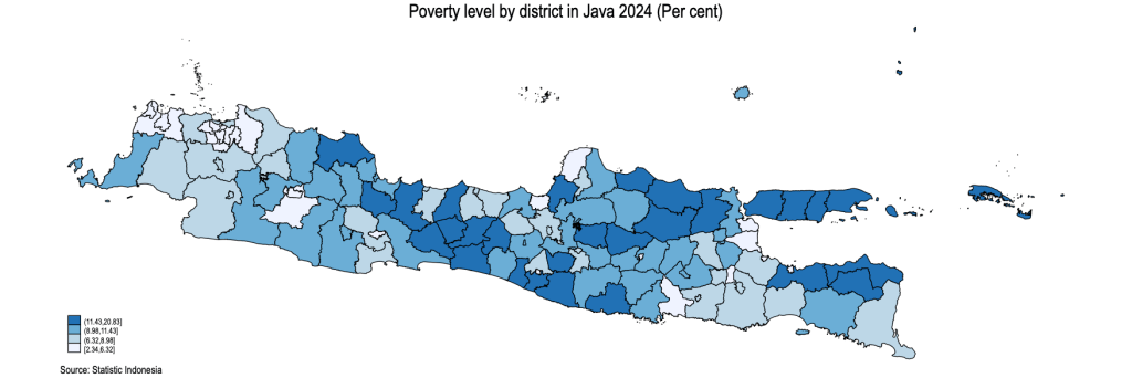
* Poverty  in Java by district level 2024 (Percent)
grmap pov2024 , title (Poverty level by district in Java 2024 (Per cent)) ///
note("Source: Statistic Indonesia")
graph save "map_poverty_adm2_java" , replace
graph export "map_poverty_adm2_java.png", as(png) name("Graph") replace

//STEP 4 : Thiessen Polygon
*Convert Shapefile thieseen polygon into dta (for spatial analysis)
copy "https://raw.githubusercontent.com/rabdulah85/public/main/java_districts_2016_tp.shp" java_districts_2016_tp.shp, replace
copy "https://raw.githubusercontent.com/rabdulah85/public/main/java_districts_2016_tp.dbf" java_districts_2016_tp.dbf, replace
copy "https://raw.githubusercontent.com/rabdulah85/public/main/java_districts_2016_tp.shx" java_districts_2016_tp.shx, replace
copy "https://raw.githubusercontent.com/rabdulah85/public/main/java_districts_2016_tp.prj" java_districts_2016_tp.prj, replace

spshape2dta java_districts_2016_tp, replace
use java_districts_2016_tp, clear
spset
sort _ID


// Merging with data poverty 2024
mmerge districtid using "https://raw.githubusercontent.com/rabdulah85/public/main/adm2_pov_java_2024.dta"
drop _merge

*Check to make sure the shapefile base is thiessen polygon
grmap pov2024, title ("Poverty level by district in Java 2024 (Per cent)") ///
note("Source: Statistic Indonesia 2025")
graph save "map_poverty_adm2_java_tp.gph", replace
graph export "map_poverty_adm2_java_tp.png", as(png) name("Graph") replace
spset 

*save 
save pov_adm2_java_tp, replace
sort _ID


//STEP 5 : Create Matrix
*Native Matrix 
spmatrix create contiguity Crownom, replace normalize(row)
spmatrix create idistance Wrownom, replace normalize(row)
spmatrix summarize Crownom //Queen contiquity matrix  with row normalization
spmatrix summarize Wrownom //Idistance matrix with row normalization
spmatrix dir 

*Matrix For Lisa 
*Create Queen Contiguity  Thiessen polygon to deal with the archipelago countries 
spmat contiguity W_java_tp using java_districts_2016_tp_shp, id(_ID) normalize(row) replace
spmat summarize W_java_tp
spmat getmatrix W_java_tp mW_java_tp
mata:
sums = rowsum(mW_java_tp)
min(sums), max(sums), mean(sums)
end
spmat summarize W_java_tp, links
spmat getmatrix W_java_tp mW_java_tp
*Save matrix 
spmat export W_java_tp using W_java_tp_temp.txt, noid replace
*Impor as dataset
import delimited W_java_tp_temp.txt, delim(space) rowrange(2) clear
* Sava as ".dta"
save W_java_tp_temp.dta, replace
* recall W_java_tp_temp.dta matrix with spatwmat (to run spatgsa)
spatwmat using W_java_tp_temp.dta, name(W_java_tp)
*check matrix
dir
spmat summarize W_java_tp
spmat summarize W_java_tp, links
*
mata:
sums = rowsum(mW_java_tp)
min(sums), max(sums), mean(sums)
end


//STEP 6 :  Check Spatial Dependence
* Open data again
use pov_adm2_java_tp, clear
*Testing for Moran I
spatgsa pov2024, w(W_java_tp) moran geary
*Testing for local spatial autocorrealtion
spatlsa pov2024, w(W_java_tp) moran id(districtid) sort

//STEP 7 :  LISA
capture program drop genmsp
*Generating the scatterplot
program genmsp, sortpreserve
version 12.1
syntax varname, Weights(name) [Pvalue(real 0.05)]

unab Y : `varlist'
tempname W
matrix `W' = `weights'
tempvar Z
qui summarize `Y'
qui generate `Z' = (`Y' - r(mean)) / sqrt( r(Var) * ( (r(N)-1) / r(N) ) )
qui cap drop std_`Y'
qui generate std_`Y' = `Z'
tempname z Wz
qui mkmat `Z', matrix(`z')
matrix `Wz' = `W'*`z'
matrix colnames `Wz' = Wstd_`Y'
qui cap drop Wstd_`Y'
qui svmat `Wz', names(col)
qui spatlsa `Y', w(`W') moran
tempname M
matrix `M' = r(Moran)
matrix colnames `M' = __c1 __c2 __c3 zval_`Y' pval_`Y'
qui cap drop __c1 __c2 __c3
qui cap drop zval_`Y'
qui cap drop pval_`Y'
qui svmat `M', names(col)
qui cap drop __c1 __c2 __c3
qui cap drop msp_`Y'
qui generate msp_`Y' = .
qui replace msp_`Y' = 1 if std_`Y'<0 & Wstd_`Y'<0 & pval_`Y'<`pvalue'
qui replace msp_`Y' = 2 if std_`Y'<0 & Wstd_`Y'>0 & pval_`Y'<`pvalue'
qui replace msp_`Y' = 3 if std_`Y'>0 & Wstd_`Y'<0 & pval_`Y'<`pvalue'
qui replace msp_`Y' = 4 if std_`Y'>0 & Wstd_`Y'>0 & pval_`Y'<`pvalue'
lab def __msp 1 "Low-Low" 2 "Low-High" 3 "High-Low" 4 "High-High", modify
lab val msp_`Y' __msp
end
//exit


genmsp pov2024, w(W_java_tp)

//check local cluster
tab msp_pov2024



//STEP 7.1 : MORAN I

* 1. Check the variable : Poverty, standardize poverty, lag_poverty and standardize lag_poverty 

summarize pov2024
summarize std_pov2024 
summarize Wstd_pov2024



* 2. Calculate Moran's I (using std_pov2024)  to display the moran I value in the scatter plot. The Moran's I value is 0.159. This number similar with Moran calculation use command spatgsa pov2024, w(W_java_tp) moran (step 6)

quietly regress Wstd_pov2024 std_pov2024
local moran_coef = _b[std_pov2024]
local moran_label : display %5.3f `moran_coef'

* 3. Quadrant-Colored Moran Scatterplot
twoway ///
  (scatter Wstd_pov2024 std_pov2024 if pval_pov2024 >= 0.05, ///
        msymbol(Oh) mcolor(gs12)) ///              <-- Not significant (Grey)
    (scatter Wstd_pov2024 std_pov2024 if pval_pov2024 < 0.05 & std_pov2024 > 0 & Wstd_pov2024 > 0, ///
        msymbol(O) mcolor(red)) ///                <-- High-High
    (scatter Wstd_pov2024 std_pov2024 if pval_pov2024 < 0.05 & std_pov2024 < 0 & Wstd_pov2024 < 0, ///
        msymbol(O) mcolor(blue*0.5)) ///           <-- Low-Low
    (scatter Wstd_pov2024 std_pov2024 if pval_pov2024 < 0.05 & std_pov2024 > 0 & Wstd_pov2024 < 0, ///
        msymbol(O) mcolor(red*0.5)) ///            <-- High-Low
    (scatter Wstd_pov2024 std_pov2024 if pval_pov2024 < 0.05 & std_pov2024 < 0 & Wstd_pov2024 > 0, ///
        msymbol(O) mcolor(ltblue)) ///             <-- Low-High
    (lfit Wstd_pov2024 std_pov2024, lcolor(blue)), ///
    yline(0, lpattern(dash) lcolor(black)) ///
    xline(0, lpattern(dash) lcolor(black)) ///
    xlabel(-4(1)4, labsize(*0.8)) ///
    ylabel(-4(1)3, angle(0) labsize(*0.8)) ///
    ytitle("{it:Spatial lag Poverty 2024}") ///
    xtitle("{it:Poverty 2024}") ///
    title("Moran Scatterplot: Poverty in Java, 2024") ///
    text(2.5 -2.0 "Moran's I = `moran_label'", place(e) fcolor(white) size(small)) ///
    legend(off) scheme(s1color)

graph export "adm2_java_oran_pov2024_quadrants.png", width(2000) replace  

/////END/////

The Output :

Poverty Map of Java Island at District Level 2024

Thiessen Polygon map, to deal with the archipelago, like Indonesia.

Moran Scatter Plot

Regio Development

Exploratory Spatial Data Analysis: STATA Application (1)

Leave a comment Cancel reply

Exploratory Spatial Data Analysis: STATA Application (1)

Share this:

Leave a comment Cancel reply